Four Bins

Chapter 11 · Milnor 1985, Strogatz 2014, Ramdas 2023

An e-value stream is a time series. "Goes up" is not a diagnosis. "Goes up then down then up" is not a diagnosis either. You need a finite set of trajectory shapes, each mapping to a different kind of system and a different next move. Dynamical systems theory provides exactly four.

Why four and not more

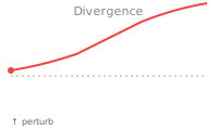
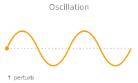
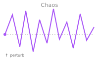
Perturb a system. Watch the response. The trajectory does one of four things:

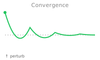
1. Convergent. The perturbation decays. The system returns to its previous state. A compensating mechanism absorbed the shock.
2. Divergent. The perturbation grows. The system moves away and keeps going. No compensating mechanism exists.
3. Oscillatory. The perturbation cycles. Two subsystems push against each other. One compensates, the other overcompensates.
4. Chaotic. The trajectory stays bounded but never repeats. Two nearby starting points diverge exponentially. Deterministic but unpredictable past a short horizon. Later chapters label this bin aperiodic, after the shape, because bounded-and-never-repeating is what a finite trace can verify; chaos in the strict sense also requires the exponential divergence.

Milnor (1985) formalized what counts as an attractor; Strogatz (2014) is the standard treatment of the classification into fixed points, limit cycles, and strange attractors. Applied to a finite observed trajectory, the four bins classify evidence behavior. They do not identify the true underlying system: a finite trace cannot prove chaos, only rule out settling and periodicity within the observed window.

Eigenvalues determine trajectory shape

Linearize the system around an equilibrium point. The Jacobian J, the matrix of first derivatives that best approximates the system near that point, has eigenvalues λ, and they determine the bin:

Five rows, three bins: convergent (decay), divergent (growth), oscillatory (rotation). Chaos requires nonlinearity and cannot appear in linear systems. For the fourth bin, you need Lyapunov exponents.

Lyapunov exponents for the nonlinear case

A Lyapunov exponent measures the rate at which two infinitesimally close trajectories diverge or converge. For an n-dimensional system, there are n Lyapunov exponents, one per dimension, ordered largest to smallest: λ₁ ≥ λ₂ ≥ … ≥ λ_n.

The largest Lyapunov exponent λ₁ determines the bin:

Eigenvalues are the linear case; Lyapunov exponents are the general case. For linear systems they coincide (the Lyapunov exponents are the real parts of the eigenvalues). For nonlinear systems, Lyapunov exponents are all you have. The four bins hold regardless.

Shape prescribes the next experiment

Observe the trajectory, match the shape, read the diagnosis, run the next experiment. Convergent: "this perturbation was absorbed, try a different node." Divergent: "this node matters, dig deeper." Oscillatory: "two things are coupled, find the coupling." Chaotic: "your decomposition is wrong, start over."

def next_experiment(classification, current_node, graph):
    """Given a trajectory classification, return the next experiment."""
    if classification == "convergent":
        # This perturbation was absorbed. Try a different node.
        return graph.least_tested_neighbor(current_node)

    elif classification == "divergent":
        # Load-bearing. Follow its dependencies.
        return graph.most_dependent(current_node)

    elif classification == "oscillatory":
        # Two subsystems fighting. Test the interface.
        return graph.interface_between(
            current_node,
            graph.oscillation_partner(current_node)
        )

    elif classification == "chaotic":
        # Decomposition is too coarse. Split into finer components.
        return graph.split(current_node)

    else:
        # Indeterminate. Collect more data at the same node.
        return current_node

Each bin maps to a graph operation: move to a neighbor, follow a dependency, test an interface, or decompose further. The bins prescribe the next move as well as classifying the last response. Chapter 12 shows how each prescription becomes an edge in the hypothesis graph.

Three questions classify any trajectory

Given a perturbation time series, three yes/no questions determine the bin:

1. Is the trajectory bounded?
   └— NO  → DIVERGENT
   └— YES → go to 2.

2. Does the trajectory settle to a fixed value?
   └— YES → CONVERGENT
   └— NO  → go to 3.

3. Does the trajectory repeat periodically?
   └— YES → OSCILLATORY
   └— NO  → CHAOTIC

Bounded? Run a Mann-Kendall trend test, a non-parametric test for a monotone trend, on the absolute values. If the trend is significantly increasing with no sign of flattening, divergent.

Settles? Compare the variance of the last third to the first third. If the late variance is significantly smaller (Levene's test, a test for unequal variances), convergent.

Periodic? Compute the power spectral density, which shows how the signal's energy distributes across frequencies. If a single frequency holds more than 40% of total power, oscillatory. If power is spread across many frequencies with no dominant peak, chaotic.

Same perturbation, four possible responses

Web server under load

A web server handles 1,000 rps. You increase to 1,500 rps and watch response time for an hour:

Same system, same perturbation, four responses depending on architecture. Chaotic is the interesting one. You're treating the whole server stack as one component when it's actually several interacting loops.

Automobile diagnostics

A mechanic suspects the alternator. She disconnects it briefly and watches the electrical system:

• Convergent: Battery voltage dips to 11.8V, recovers to 12.6V when the alternator reconnects. The battery absorbed the perturbation. The alternator is redundant at current draw.
• Divergent: Voltage drops steadily. The radio dims, the dashboard flickers, the engine stalls. The alternator was the only power source at this draw level. Everything downstream cascaded.
• Oscillatory: Voltage swings between 11V and 14V with a 2-second period. The voltage regulator and the alternator are fighting. One compensates, the other overcompensates. The fault is in the interface: the regulator. The alternator itself is fine.

Chaos is rare in simple electrical circuits. Three bins cover most automotive faults. But engine management systems have enough interacting control loops (fuel injection, ignition timing, variable valve timing, turbo boost) that a single sensor failure can produce bounded but aperiodic behavior no single root cause explains.

Clinical trial

A drug trial measures blood pressure over 18 months. The perturbation is the drug. The trajectory is the patient's BP over time:

• Convergent: BP drops from 150 to 130 in the first month, stabilizes. The drug works and the effect is stable.
• Divergent: BP drops to 130, then creeps back to 145, then 155, then 160. The body adapts. The drug works in the snapshot window but the compensatory response overwhelms it. This is Vioxx (one of chapter 9's three snapshot cases).
• Oscillatory: BP swings between 125 and 155 with a monthly period. The drug suppresses BP for two weeks, the body overshoots for two weeks, the drug wins again. The interface is the feedback loop between drug and compensatory mechanism.
• Chaotic: BP stays between 120 and 160 but follows no pattern. The drug interacts with diet, exercise, stress, sleep, and other medications to produce bounded but unpredictable responses. A single drug-response model is the wrong decomposition; factor out the other variables first.

A 9-month snapshot of the divergent case shows "BP dropped, drug works." The 18-month e-value trajectory shows the evidence reversing. The bin tells you why: the compensatory response overwhelms the drug, and that response is the mechanism to investigate.

Code: trajectory classifier

The implementation follows the decision tree: check boundedness, then settling, then periodicity.

import micropip
await micropip.install('scipy')

import numpy as np
from scipy import stats, signal

def classify_trajectory(ts, alpha=0.05):
    """Classify a perturbation-response time series into four bins."""
    ts = np.asarray(ts, dtype=float)
    n = len(ts)

    if n < 30:
        return {'bin': 'indeterminate', 'evidence': {'reason': 'too few observations'}}

    evidence = {}

    # Step 1: Is it bounded? (Mann-Kendall trend on |x|)
    abs_ts = np.abs(ts - np.mean(ts[:n // 10]))
    mk_tau, mk_p = stats.kendalltau(np.arange(n), abs_ts)
    evidence['trend_tau'] = mk_tau
    evidence['trend_p'] = mk_p

    late_start = 3 * n // 4
    late_tau, late_p = stats.kendalltau(
        np.arange(n - late_start), abs_ts[late_start:]
    )

    if mk_tau > 0 and mk_p < alpha and late_tau > 0 and late_p < alpha:
        return {'bin': 'divergent', 'evidence': evidence}

    # Step 2: Does it settle? (variance ratio, Levene's test)
    third = n // 3
    var_early = np.var(ts[:third])
    var_late = np.var(ts[-third:])

    if var_early > 0:
        lev_stat, lev_p = stats.levene(ts[:third], ts[-third:])
        var_ratio = var_late / var_early
        if var_ratio < 0.25 and lev_p < alpha:
            return {'bin': 'convergent', 'evidence': evidence}

    # Step 3: Is it periodic? (Welch PSD, peak fraction)
    freqs, psd = signal.welch(ts - np.mean(ts), nperseg=min(256, n // 2))
    total_power = np.sum(psd)
    if total_power > 0:
        peak_idx = np.argmax(psd[1:]) + 1
        peak_fraction = psd[peak_idx] / total_power
        if peak_fraction > 0.40:
            return {'bin': 'oscillatory', 'evidence': evidence}

    return {'bin': 'chaotic', 'evidence': evidence}


# Demo: one of each
np.random.seed(42)
t = np.linspace(0, 10, 500)

conv = 5.0 * np.exp(-0.5 * t) + np.random.normal(0, 0.1, len(t))
div  = 0.1 * np.exp(0.3 * t)  + np.random.normal(0, 0.1, len(t))
osc  = 3.0 * np.sin(2 * np.pi * 0.5 * t) + np.random.normal(0, 0.3, len(t))

def lorenz_x(n_steps=500, dt=0.02, sigma=10, rho=28, beta=8/3):
    x, y, z = 1.0, 1.0, 1.0
    xs = []
    for _ in range(n_steps):
        dx = sigma*(y-x); dy = x*(rho-z)-y; dz = x*y-beta*z
        x += dx*dt; y += dy*dt; z += dz*dt
        xs.append(x)
    return np.array(xs)

chaos = lorenz_x()

for name, series in [("convergent", conv), ("divergent", div),
                       ("oscillatory", osc), ("chaotic", chaos)]:
    result = classify_trajectory(series)
    print(f"{name:<12} -> {result['bin']}")

Three statistical tests in sequence. The simplicity is deliberate. A classifier that requires tuning 20 parameters costs more to calibrate than the trajectory is worth reading. Three tests, three thresholds, four bins.

Where the classifier fails

Transient classification. A system divergent in the first 100 observations may converge by observation 500. The classifier sees whatever window you give it. Fix: run the classifier on a rolling window and watch whether the bin itself flips. If it does, you're in the transient regime and need more data.

Oscillatory vs. chaotic at the boundary. A system with a dominant frequency plus significant broadband noise will land on one side or the other of the 40% threshold. This boundary is the least important one. Both bins indicate coupling between subsystems; the difference matters for prediction (oscillatory is predictable, chaotic is not) but not for the next experiment (both say "test the interface" or "decompose").

E-value trajectories have the same four shapes

The e-value stream from Chapter 10 is itself a time series. Apply the classifier to it.

An e-value that converges to a high value: evidence accumulated and stabilized. Redirect budget elsewhere.

An e-value that diverges: evidence piling up monotonically. This is the normal "success" mode for anytime-valid inference.

An e-value that oscillates: evidence swings back and forth periodically. This is the signature of Boeing's MCAS. The hypothesis is incomplete rather than wrong: it captures one half of a coupled pair.

An e-value that looks chaotic: evidence is bounded but never settles and never repeats. Your betting strategy is poorly matched to the system's dynamics. You are testing at the wrong level of abstraction, like asking "does the server have a latency problem?" when the real question requires decomposing into cache, queue, and retry-loop subproblems.

Bins classify nodes; kill conditions generate edges

The classification table has a column labeled "Next experiment." But nothing in the eigenstructure or the Lyapunov exponent tells you which node to test, which dependency to probe, or how to decompose. The four bins tell you what kind of response you got. They do not tell you what to do next.

That mapping is the claim of chapter 12. Each bin produces a kill condition: a specific, testable statement about what would have to be true for the diagnosis to be wrong. The kill condition generates the next edge in the hypothesis graph.

Exercises

💻 marks exercises meant for a keyboard. ★ marks open-ended problems with no single right answer.

11.1 Why can a linear system never land in the chaotic bin? Answer in two sentences using the eigenvalue table, then say which single number replaces the eigenvalues when the system is nonlinear.

11.2 Bin each trajectory and, using the prescription table, name the next experiment. (a) A group chat erupts after someone posts a hot take; message rate spikes to 40 per minute and is back to its usual 2 per minute by evening. (b) A student's sleep debt grows every week of the term, and each week's deficit is larger than the last. (c) Two roommates share a thermostat; the apartment cycles between 18° and 24° with a reliable daily period. (d) Your phone's battery level over a festival weekend stays between 5% and 80% with no discernible pattern and no repetition.

11.3 Pick a system you touch daily (your inbox, a sourdough starter, a shared codebase, your commute) and design one concrete perturbation for it. Predict its bin. Then, for each of the other three bins, state what fact about the system's architecture would have to be true for the trajectory to land there instead. You now hold four rival hypotheses about one system; note that the perturbation was designed before any of them was favored.

11.4 💻 Generate a damped oscillation, 5 * np.exp(-0.3 * t) * np.sin(2 * np.pi * 0.5 * t) plus a little noise, and feed it to classify_trajectory. The eigenvalue table calls damped oscillation convergent. If the classifier disagrees, trace which of the three tests fired first, adjust exactly one threshold until the answer matches the table, then rerun the chapter's four demo series. What did your fix break, and what does that trade-off teach about the 40% threshold?

11.5 ★ Export any personal time series you can get your hands on: screen time, spending, running pace, caffeine intake. Classify the full series, then classify it again on rolling windows a quarter of its length. If the bin flips between windows, decide whether you are watching a transient regime or an artifact of window size, and design the observation that would tell those apart.

Sources